Lab 6 - Numpy

This is not available yet. It will be released when it is assigned.

---

Due Date and Links

• Lab due on your scheduled lab day

• Lab accepted for full credit until Monday, March 9, 11:59 pm Eastern

• Direct autograder link https://autograder.io/web/project/3542

---

In this lab, you are going to use your newly acquired numpy skills to build computer vision algorithms.

Background

Computer vision is a subset of artificial intelligence that operates on images and videos, allowing a computer to “see” the same things you do. It is used in technology such as facial recognition, smart photo editing, and self-driving cars. Many computer vision algorithms can be implemented with numpy.

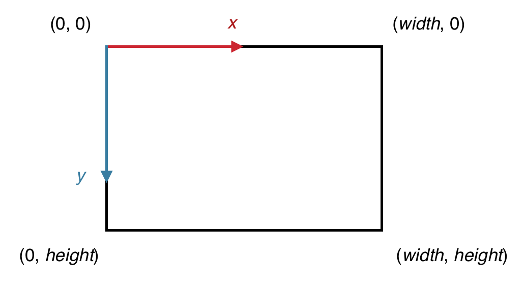
The Coordinate System

In computer graphics, it is common to represent an image in a coordinate system where the x axis is directed to the right, but the y axis is directed downward, so that the origin is in the top left corner. And so if the image is of size 100 pixels × 100 pixels, the pixel at coordinate (0,0) would be located in the top left corner, the pixel at coordinate (99,0) would be in the top right corner, the pixel at coordinate (0,99) would be in the bottom left corner and the pixel at coordinate (99,99) would be in the bottom right corner. Here’s a general diagram:

Representation of a Single Pixel

Each pixel has a specific color. Color is often represented with three numbers in computing. Red, green, and blue are the primary colors that are mixed to display the color of a pixel on a computer monitor. Nearly every color of emitted light that a human can see can be created by combining these three colors in varying levels. And so we can set the color of a pixel by specifying the amount of red, green and blue we want.

The intensity of red, green and blue ranges from 0 to 255 each, with 0 meaning “none of that color” and 255 meaning “lots of that color”. Thus, the RGB (red-green-blue) representation of a color is three such values: first the intensity of red, then the intensity of green, and finally blue. For example, a few colors are illustrated below:

• Red: (255, 0, 0)  
• Pink: (255, 0, 255)  
• Khaki: (195, 176, 145)  

Representation of an Image

We might think of an image as a two-dimensional structure of pixels, with a pixel uniquely identified by its row and column. In computer vision, we often call each dimension an axis. But since each pixel actually has three components (R, G, and B), we can think of a third “color” axis as well. Thus we can think of one full-color image as three “special images” stacked on top of each other: one for the red intensities, one for the green intensities, and one for the blue intensities. Each of these “special images” is called a color channel, or just channel. This image representation scheme is depicted below:

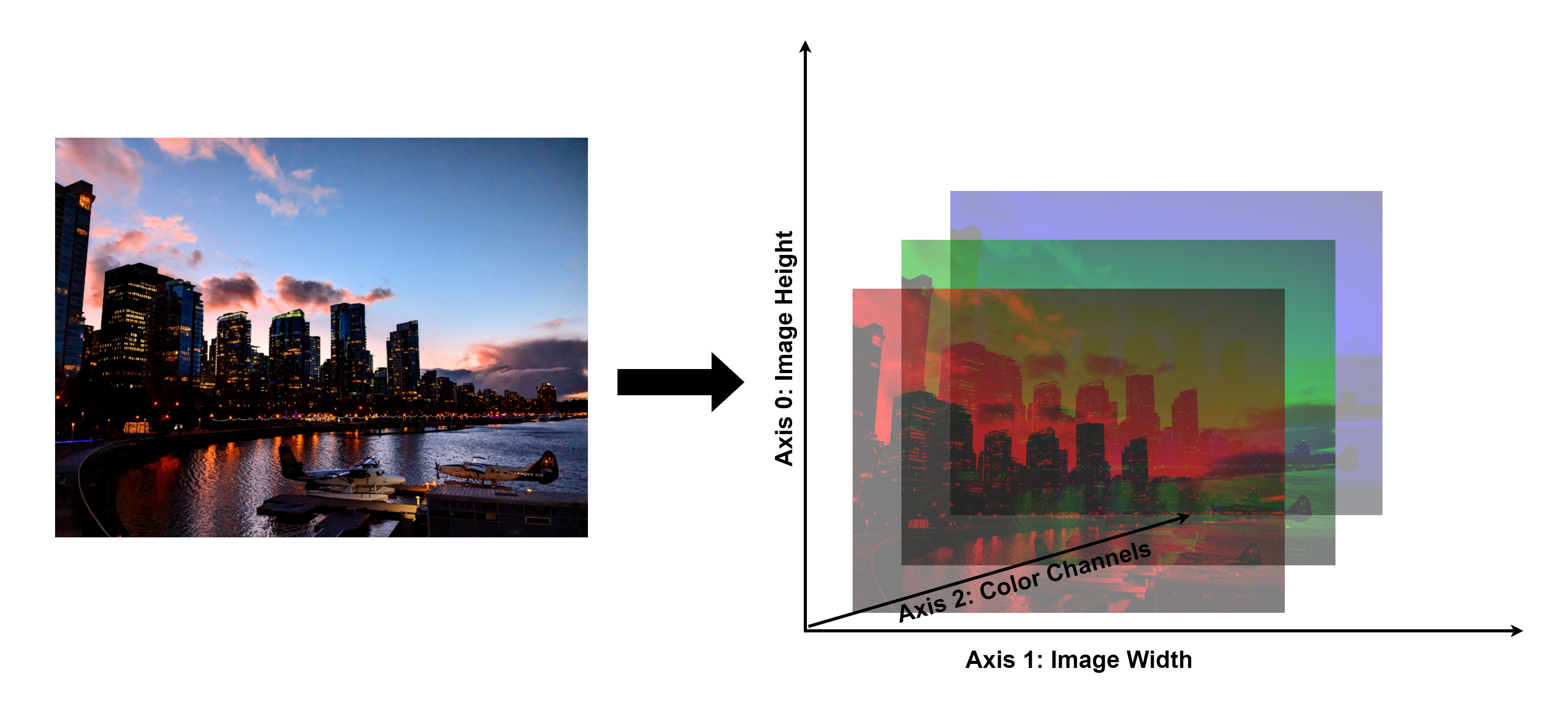
The entire image can be represented as a three-dimensional numpy array, where axis 0 represents the height of the image (number of rows), axis 1 represents the width of the image (number of columns), and axis 2 represents the three color channels (red, green, blue). We can uniquely identify a single number in this structure by specifying its row, its column, and which color channel it is in (R, G, or B). Each individual number represents the intensity of a certain color at a certain pixel in the image.

In the starter code, you will see that images have the type NDArray[np.uint8]. The NDArray part means that the structure is an array with some number of dimensions. We state in the Requires clause that the structure must actually have three dimensions. uint8 means the array contains unsigned (no negative values allowed) 8-bit integers; briefly, this is an integer type where the value is restricted to between 0 and 255, inclusive.

NOTE: For certain functions, we’ll represent images as NDArray[np.float64] – a 3D array of floats. See the function hints section below for more details on why.

Starter Files

You can download the starter files using this link. The starter files download includes the following:

• computer_vision.py: this is the file you will be coding in. It already contains function stubs for each of the image transformations you will be doing.
• example.jpg, blend1.jpg and blend2.jpg: these are the images that you will be transforming.

How to Submit

IMPORTANT: For all labs in EECS 183, to receive a grade, every student must individually submit the Lab Submission. Late submissions for Labs will not be accepted for credit.

• Once you receive a grade of 10 of 10 points from the autograder you will have received full credit for this lab.

Functions to Implement

Today, you are going to implement 7 computer vision algorithms:

• Red Channel Isolation: display just the red intensities of the image
• Blue Channel Isolation: display just the blue intensities of the image
• Green Channel Isolation: display just the green intensities of the image
• Grayscale: convert a color image into black-and-white
• Negative: convert an image into the negative of itself
• Brightness: change the brightness of an image to make it lighter or darker
• Blending: blend two images together

See the below sections for more details on how to implement these functions!

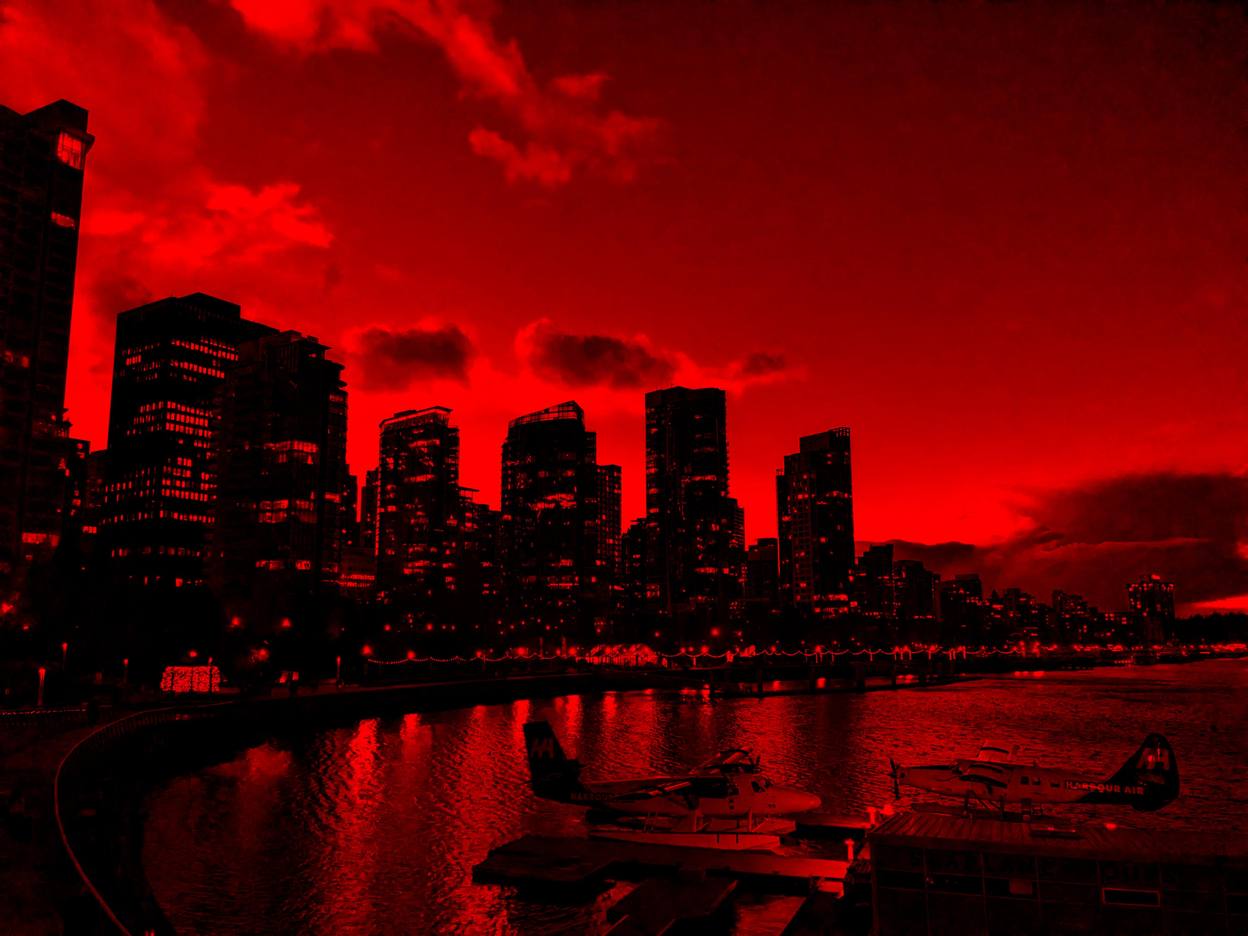
Functions 1, 2 and 3: Isolating Color Channels

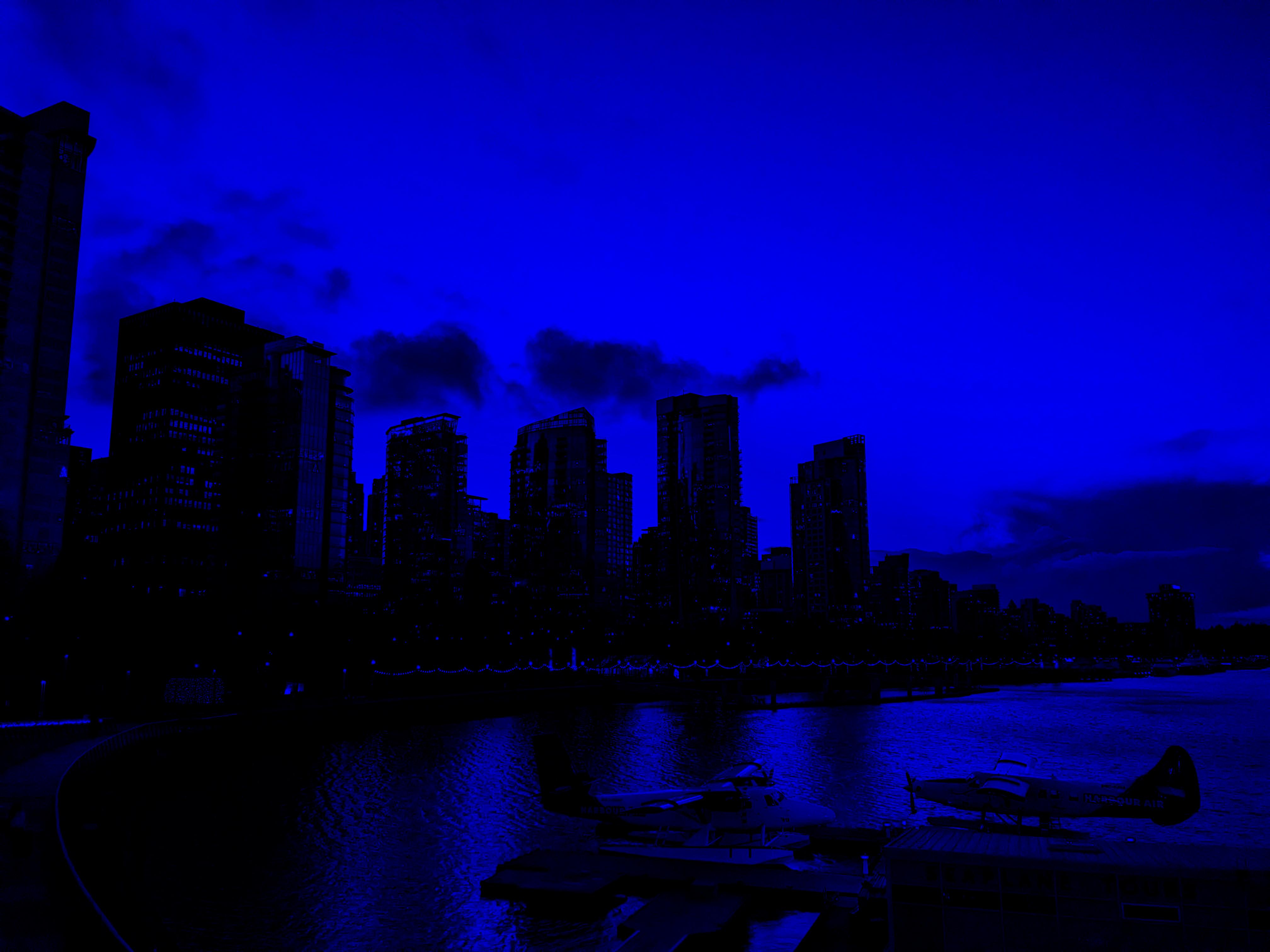
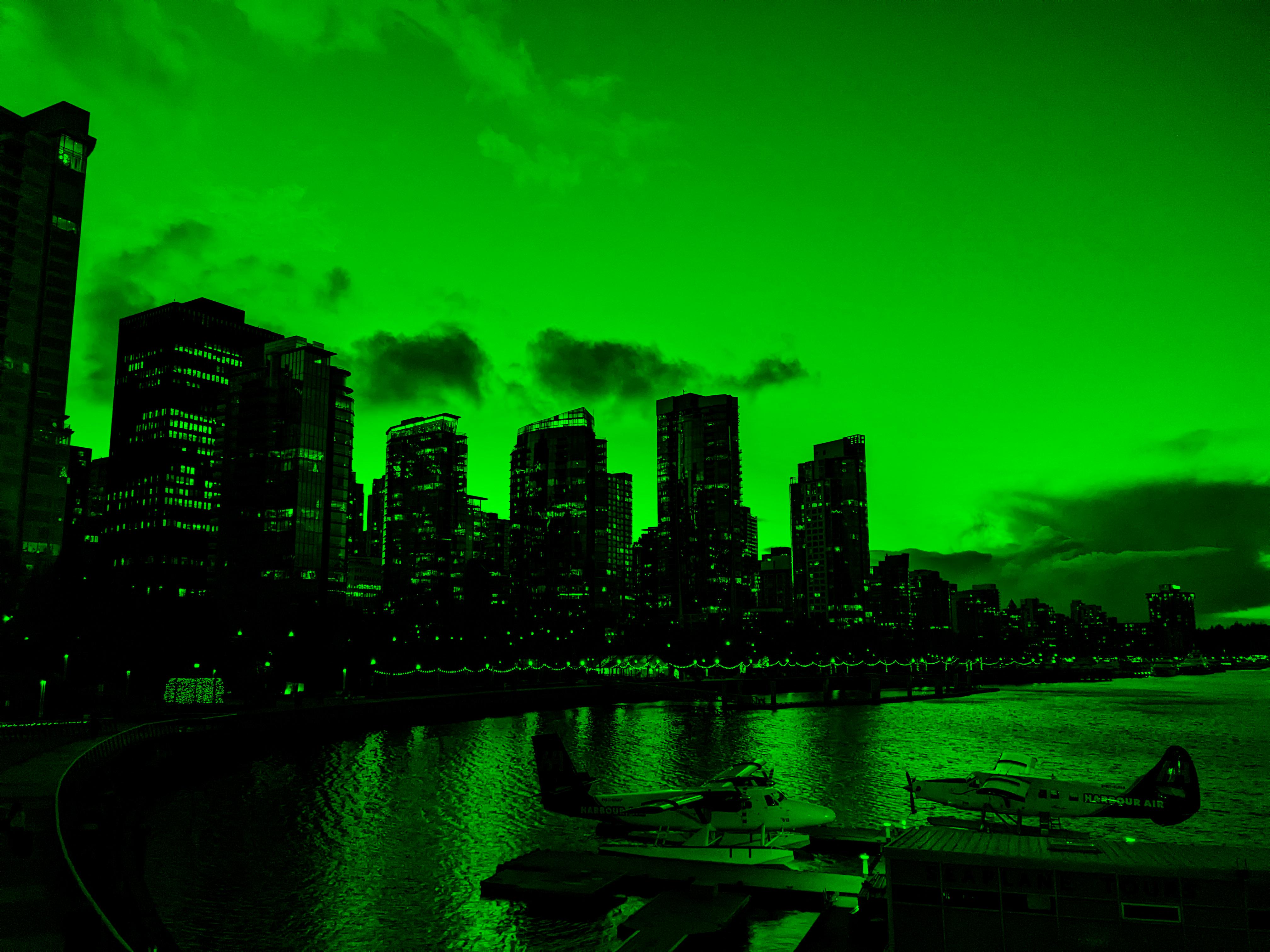
For show_red, show_green, and show_blue, we’d like to “isolate” each color channel, respectively. For example, in show_red, we’d like to see only the red parts of the image, with the green and blue parts set to black (intensity 0). Implement show_red, show_green, and show_blue accordingly.

Note: The easiest way to do this is with slicing and assignment. However, this would result in a mutation of the original image (passed in as an argument), which would violate the “Modifies: Nothing” clause. Thus the first step in each of these functions should be to make a copy of the input image using the copy method, and work with that copy instead.

Working with example.jpg, your results should look like the images below. The first image is the original, followed by the red, green, and blue isolated channel versions.

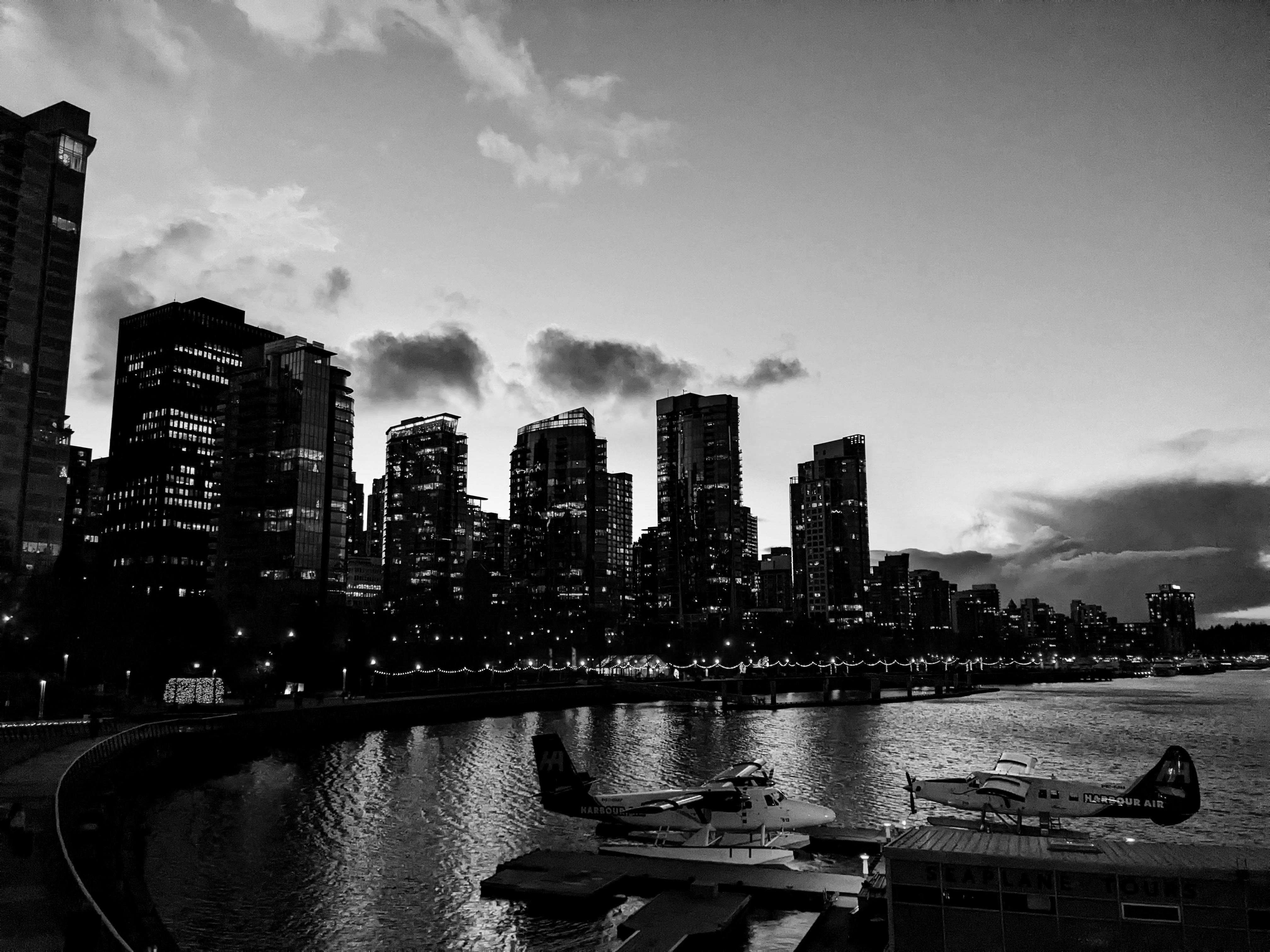
Function 4: Grayscale

For a grayscale image, each pixel only has one intensity value, representing how light or dark that pixel is. A pixel with intensity 0 is black, a pixel with intensity 255 is white, and pixels with intensities in between are shades of gray. To convert a color image to a grayscale image, we need to combine the three color channels (red, green, and blue) into one channel. That is, imagine “flattening” the three color channels into one channel. How will we do this? We can simply take the mean of the intensities of the red, green, and blue pixels at each location. For example, if a pixel has RGB values of (100, 150, 200), then the grayscale intensity for that pixel would be (100 + 150 + 200) / 3 = 150.

Implement to_grayscale accordingly. Note:

• The mean function returns an array of np.float64 values; this makes sense, since the mean of integers is (can be) a float. Thus, to match the required return type, you’ll need to use the astype function.
• Since we’re combining the three color channels into one, we’re left with just two dimensions: height and width. Thus, the returned array should be a 2D structure.

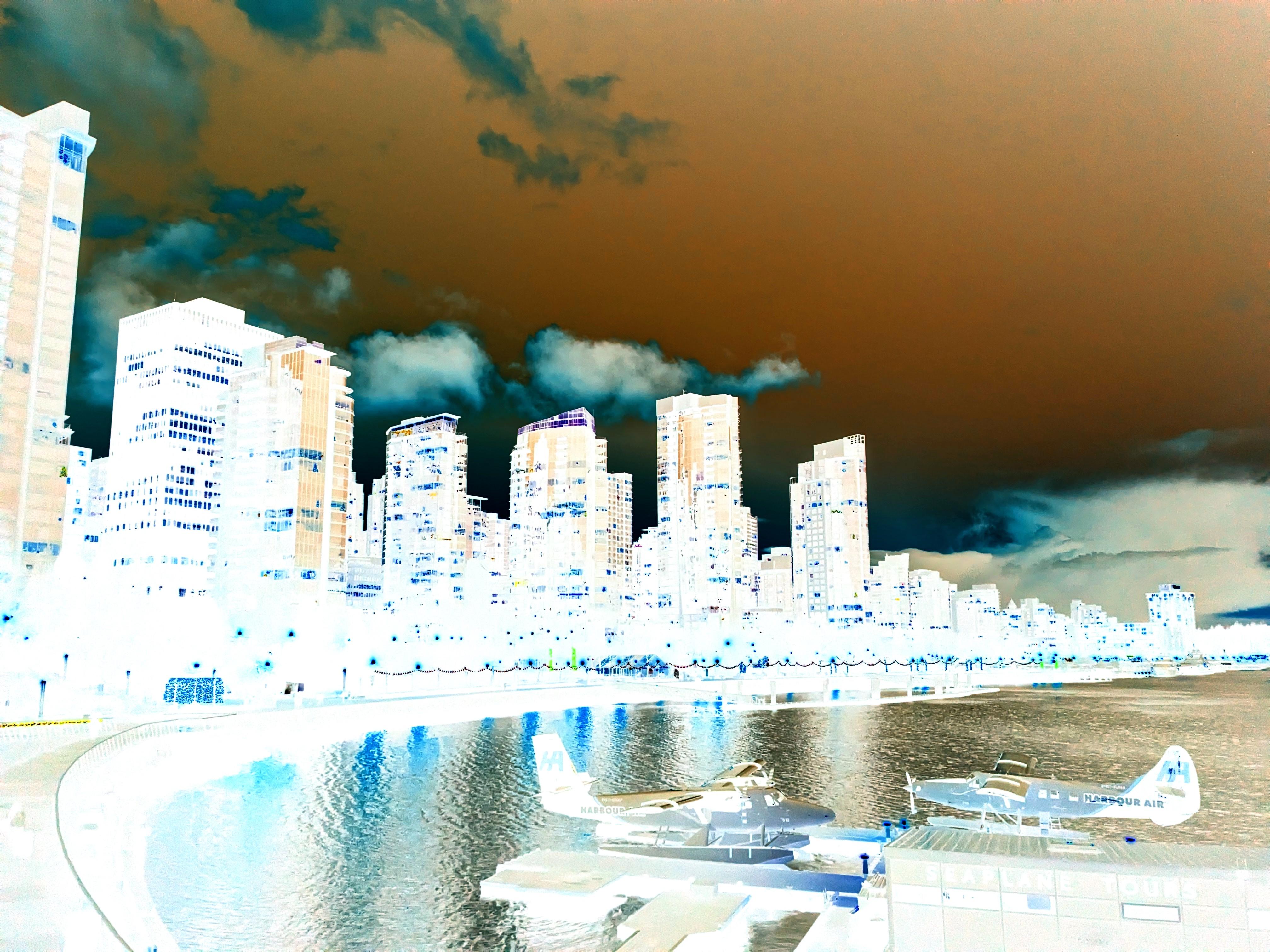
Function 5: Negative

A photo negative is like the opposite of an original photo - light becomes dark, dark becomes light, red becomes blue, etc. However, creating a negative does not just mean multiplying the value of each color’s intensity by -1: remember, pixel intensities have to be between 0 and 255! Rather, we find the “opposite” of each pixel’s intensity: 0 becomes 255, 1 becomes 254, and so on. Implement image_negative accordingly.

Function 6: Brightness

Adjusting the brightness of an image involves increasing intensities of all the pixels by a certain amount. In other words, we’re adding a certain constant, which is passed in as a parameter, to every element in the image array.

Before we say more about brightness, we need to understand the concepts of overflow and underflow. As discussed above, the value of uint8 is restricted to between 0 and 255, inclusive. What happens if we try to add 10 to a pixel with intensity 250? The answer is that the value “overflows” and wraps around back to 0. Thus, 250 + 10 = 4 when we’re dealing with a value of type uint8! Similarly, if we try to subtract 10 from a pixel with intensity 5, the value “underflows” and wraps around back to 255. For example, 5 - 10 = 251 when the type is uint8.

We need to handle overflow and underflow issues when adjusting brightness. Overflow can happen when we have very bright pixels (intensities close to 255) and we try to increase the brightness further. Underflow can happen when we have very dark pixels (intensities close to 0) and we try to decrease the brightness (with a negative value).

So we need to cap the maximum value at 255 and the minimum at 0. Implement adjust_brightness as follows:

1. Use astype to convert the image array to int16 – this is a signed 16-bit integer, meaning that it can hold values between -32,768 and 32,767. This is way more than we need, but there’s no such thing as int9, for example, so this is the smallest type that will work.
2. Add the brightness value to the image.
3. Use the clip function to ensure that all values are between 0 and 255.
4. Use astype to convert the image array back to uint8 before returning.

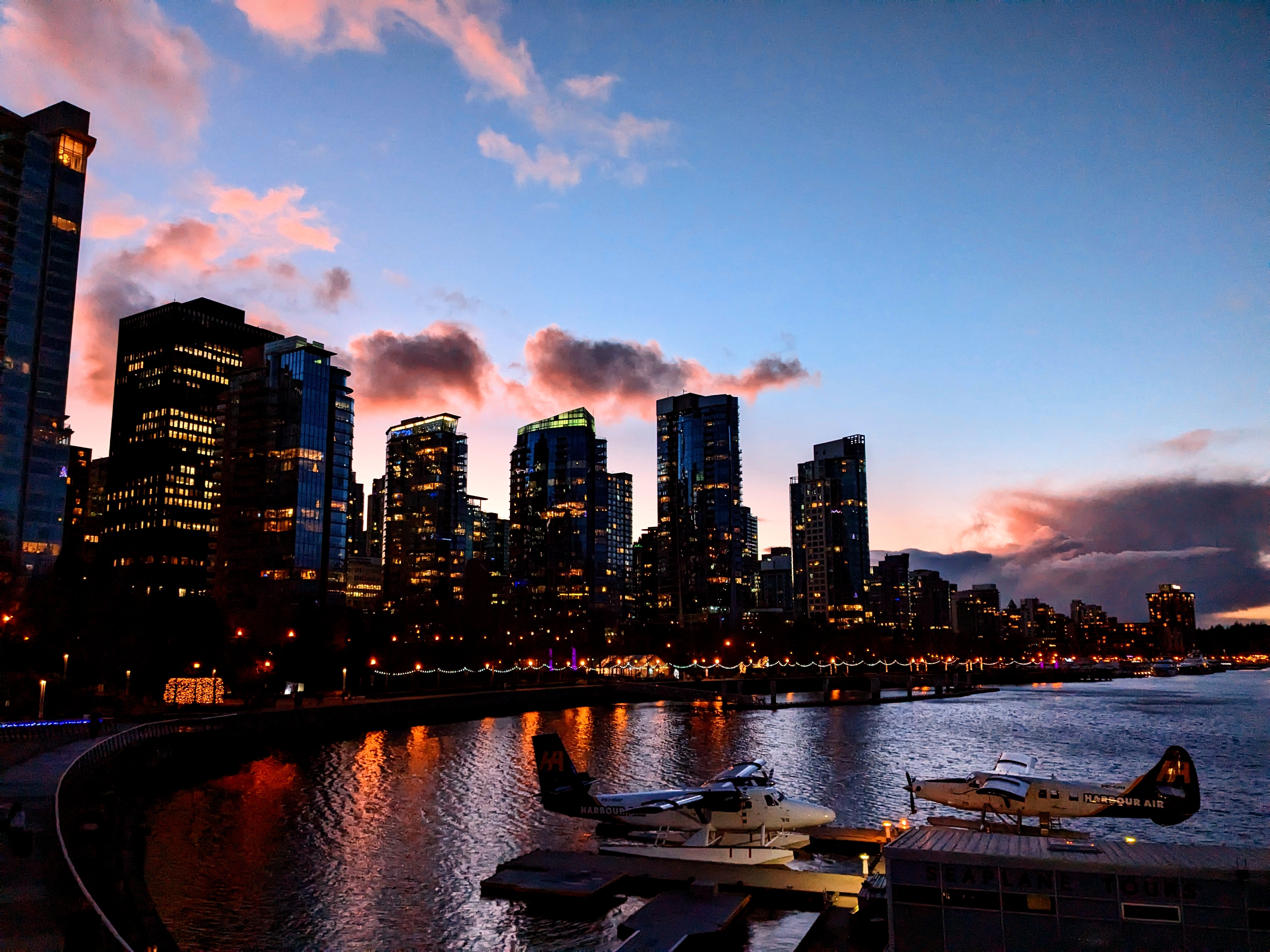
Function 7: Blending

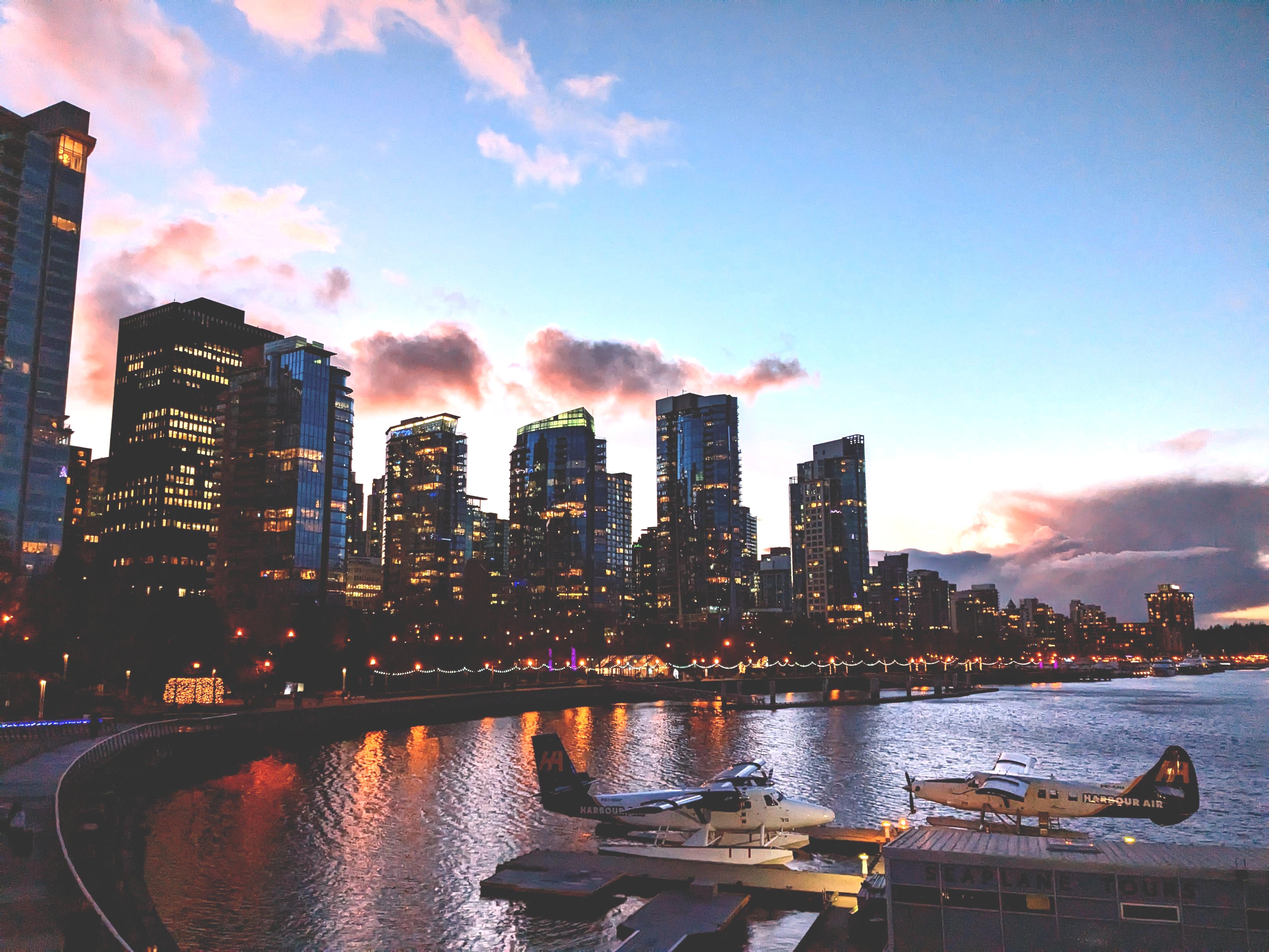
Blending two images should look something like this:

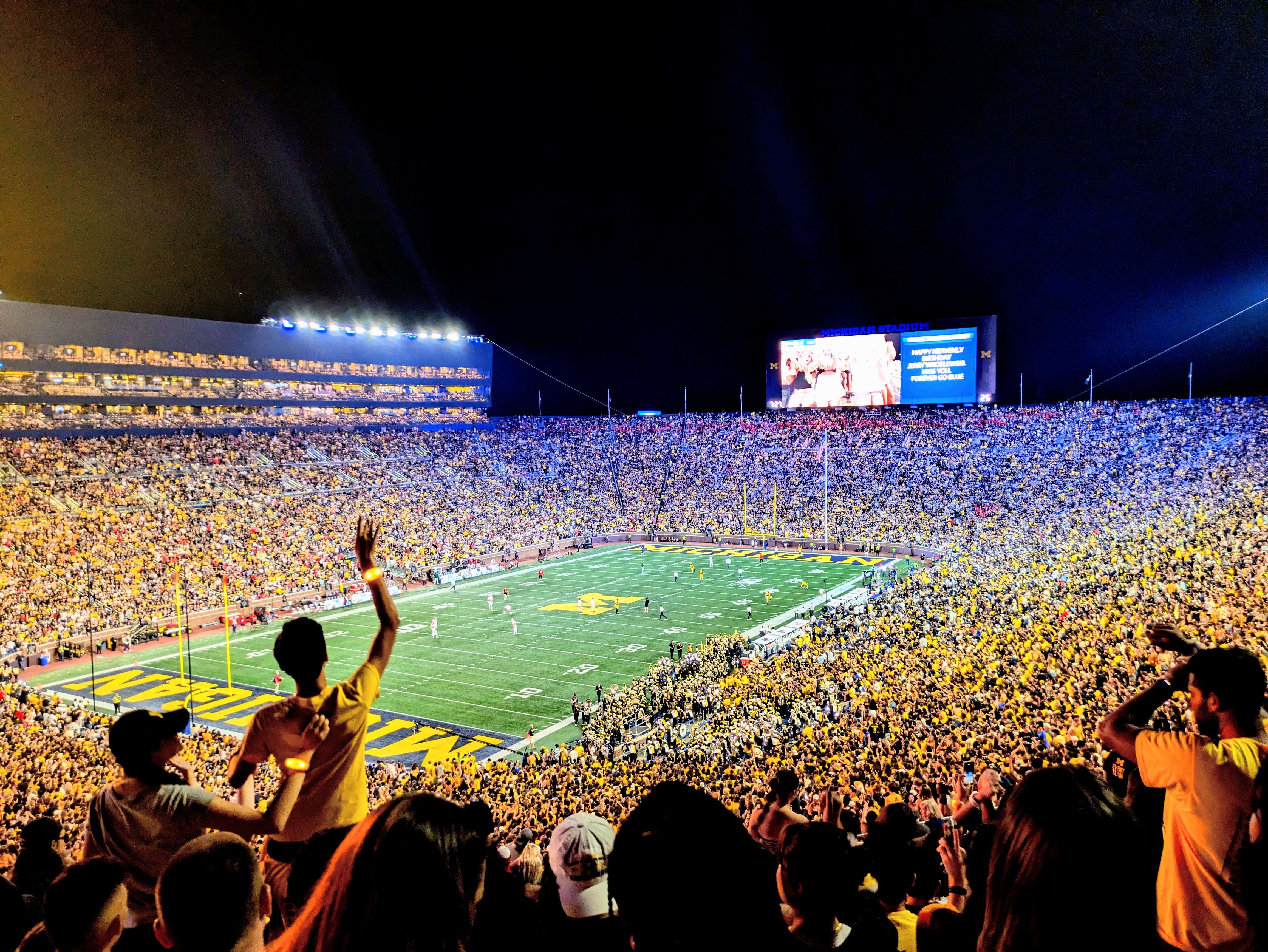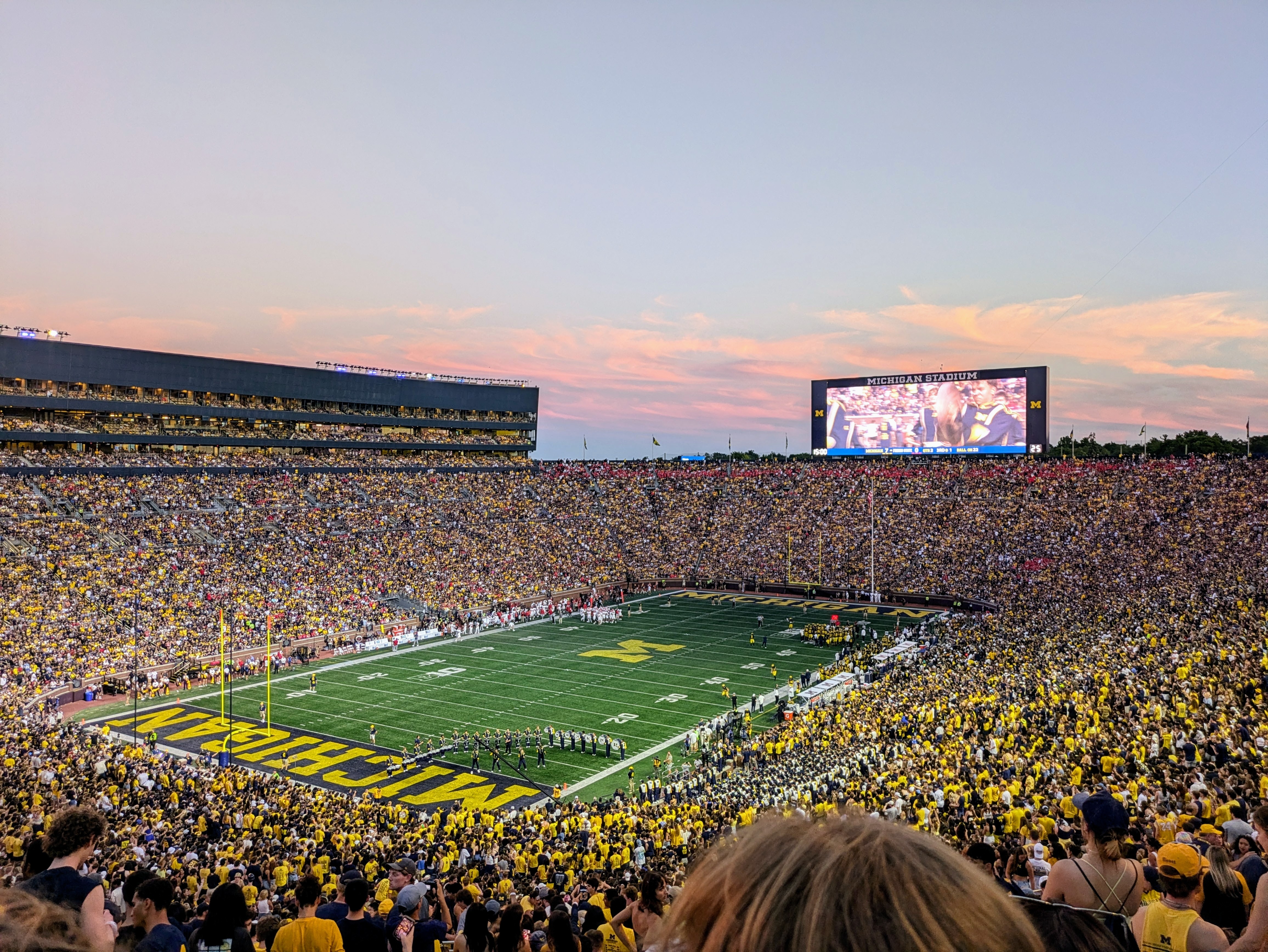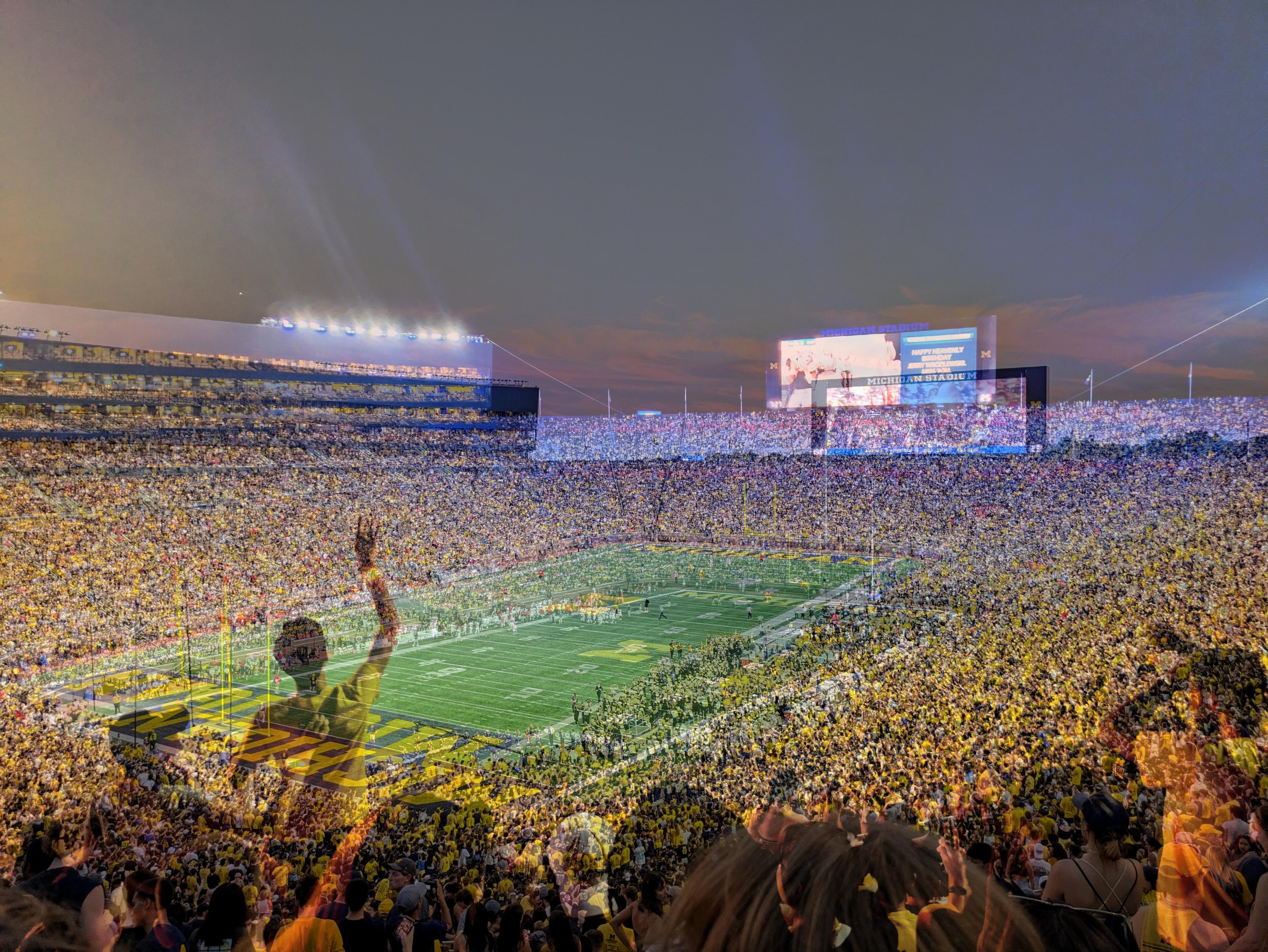
In order to blend two images, we use the following equation: blended = alpha * img1 + (1 - alpha) * img2

alpha is a decimal value between 0 and 1 that tells us how much of each image we see. If alpha is 1, then we only see image 1. If alpha is 0, we only see image 2. If alpha is 0.5, then we see half of image 1 and half of image 2.

As with adjust_brightness, for blend_images here we’ll need to think carefully about types. Before doing anything else, your function should convert the two input images to use float32. If we don’t convert, then multiplying the uint8 values by alpha will result in float64 values instead. The ultimate behavior would be the same, but the float64 type takes up twice as much memory as float32. We don’t need that extra space, so we’ll explicitly convert to float32 instead of allowing an implicit conversion to float64. Across a large image, the memory savings can be significant.

After converting to float32, perform the blending operation above, clip, and then astype back to uint8 before returning.

Try Some More

When you finish the lab, you might find it fun to play around with images of your own, or even write additional image processing functions! Also note the imwrite function used in main, to save the numpy array images to files.

Photos by Krithika Venkatasubramanian (‘26)